Chris Wendler, 11/21/24
This material is evolving. If you have questions or suggestions feel free to reach out to me. More here.
Let’s start by recapitulating the ADAM update $\Delta W$and the spectral condition that we are trying to achieve.
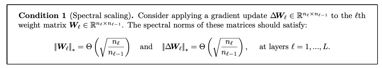
From the spectral condition for feature learning paper we know that in order to achieve feature learning our weight updates $\Delta W$ have to satisfy Condition 1:
From the ADAM paper:
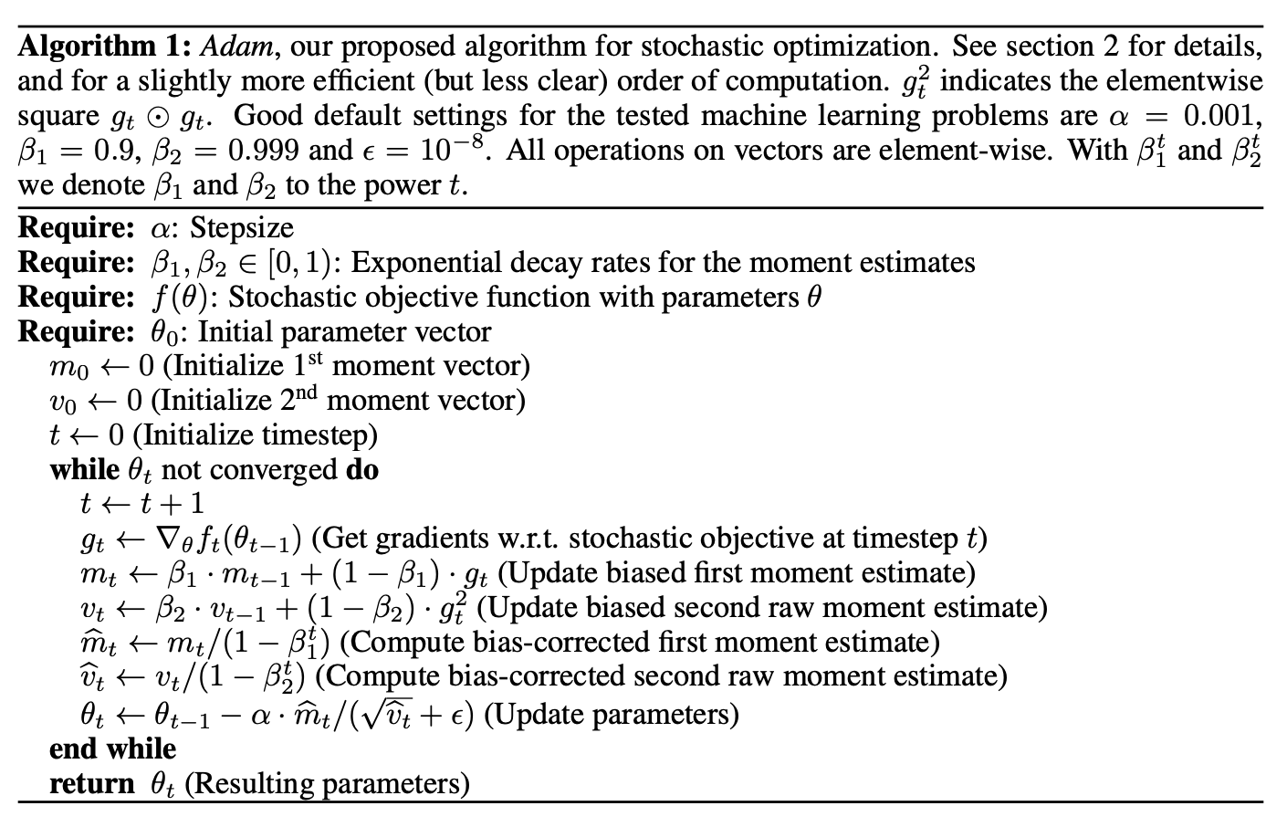
Thus, we have
\[\Delta W = \alpha \cdot \widehat{m}_t/(\sqrt{\widehat{v}_t}+\epsilon).\]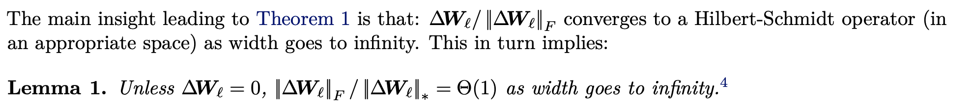
Intuition: \(\|\Delta W\|_2^2 = tr(\Delta W \Delta W^T) = \sum_i \sigma_i^2\) (follows from trace rules). Thus, \(\frac{\|\Delta W\|_2^2}{\|\Delta W\|_*^2} = 1 + \underbrace{\sum_{k=2}^n \frac{\sigma_k^2}{\sigma_1^2}}_{\Theta(1)\text{ for }n\to\infty}\).
Importantly, once we have the order of the spectral norm of \(\Delta W\), we can simply set the learning rate such that Condition 1 is satisfied.
Recall
\[\begin{aligned} & m_t = \beta_1 m_{t-1} + (1 - \beta_1) g_t \\ & v_t = \beta_2 v_{t-1} + (1 - \beta_2) g_t^2 \\ &\widehat{m}_t = m_t / (1 - \beta_1^t)\\ &\widehat{v}_t = v_t / (1 - \beta_2^t)\\ &\Delta W = \alpha \cdot \widehat{m}_t/(\sqrt{\widehat{v}_t}+\epsilon). \end{aligned}\] \[\text{For }t\to\infty \text{ both } \widehat{m}_t \to m_t \text{ and } \widehat{v}_t \to v_t \text{ because } \beta_1, \beta_2 \in [0, 1).\]Therefore, we only need to consider \(m_t\) and \(v_t\). For taking the limit \(t \to \infty\) it is easier to work with their closed form, which can be obtained via telescoping:
\[\begin{aligned} m_t &= \beta_1 (\beta_1 m_{t-2} + (1-\beta_1)g_{t-1}) + (1-\beta_1)g_t\\ &= \beta_1^2 m_{t-2} + \beta^1_1 (1 - \beta_1) g_{t-1} + \beta^0_1 (1 - \beta_1) g_t \\ &\dots \\ &= (1-\beta_1) \sum_{i=1}^t \beta_1^{t-i} g_i \\ \end{aligned}\]The same can be done for \(v_t\), which results in
\[\begin{aligned} v_t &= (1-\beta_2) \sum_{i=1}^t \beta_2^{t-i} g_i^2. \end{aligned}\]Both \(m_t\) and \(v_t\) are geometric series of i.i.d. random variables.
Proof
In order to proof this we are going to insert an extra zero, which will simplify the analysis:
\[\begin{aligned} \sum_{i = 1}^n \beta^i X_i &= \sum_{i = 1}^n \beta^i (X_i - \mathbb{E}[X_i] + \mathbb{E}[X_i])\\ &= \sum_{i = 1}^n \beta^i (X_i - \mathbb{E}[X_i]) + \sum_{i = 1}^n \beta^{i}\mathbb{E}[X_i]. \end{aligned}\]The second term now becomes
\[\begin{aligned} \sum_{i = 1}^n \beta^{i}\mathbb{E}[X_i] &= \mu \frac{1 - \beta^{n+1}}{1 - \beta}. \end{aligned}\]which in the limit is
\[\lim_{n \to \infty} \mu \frac{1 - \beta^{n+1}}{1 - \beta} = \frac{\mu}{1- \beta}.\]The first term now is a sum of i.i.d. variables with zero mean,
\[\text{i.e., }Y_i = \beta^i (X_i - \mathbb{E}[X_i]) \text{ with } \mathbb{E}[Y_i] = 0.\]Thus, by applying the law of large numbers we obtain that the first term converges to zero (in probability). This concludes the proof
\[\lim_{n \to \infty} \sum_{i = 1}^n \beta^i X_i = 0 + \mu/(1-\beta).\]Applying our Lemma 2 to \(m_t\) and \(v_t\) for \(t \to \infty\) results in
\[\begin{aligned} m &= \lim_{t \to \infty} m_t = \mathbb{E}[g],\\ v &= \lim_{t \to \infty} v_t = \mathbb{E}[g^2] = Var[g] + \mathbb{E}[g]^2, \end{aligned} \\ \text{and }\Delta W \text{ approaches }\alpha \frac{m}{\sqrt{v} + \epsilon}.\]Notice that while $m$ and $v$ are matrices all operations were always applied entry-wise.
Now, assuming that the entry-wise expectation and variance of the gradients are of constant order
\[\mathbb{E}[g_{ij}] = \mu_{ij} = \Theta(1) \text{ and } Var[g_{ij}] = \sigma_{ij}^2 = \Theta(1),\]it is straightforward to compute the order of the Frobenius norm
\[\|\Delta W\|_2 = \Theta(\sqrt{\alpha ^2 n_{\ell} n_{\ell-1}}).\]Thus, by Lemma 1 from above the spectral norm also is of the same order
\[\|\Delta W\|_* = \Theta(\sqrt{\alpha ^2 n_{\ell} n_{\ell-1}}) = \Theta(\alpha \sqrt{n_{\ell} n_{\ell-1}}).\]Note: I am not sure how realistic this assumption is. I mainly needed it to get the matching lower bound for the Frobenius norm. The upper bound can be done also without this assumption by using Jensen’s inequality. I would be grateful about some input here.
Let’s consider the typical case in which \(n_{\ell} = n_{\ell - 1} = n\). As a result, we have \(\Delta W = \Theta(\alpha n)\), which is required to be \(\Theta(1)\) by Condition 1. Therefore, \(\alpha\) must be in \(\Theta(\frac{1}{n})\).
Let’s consider the typical case in which \(n_{\ell} = n\) and \(n_{\ell - 1} = c\) (some constant). As a result, we have \(\Delta W = \Theta(\alpha \sqrt{cn}) = \Theta(\alpha \sqrt{n})\), which is required to be \(\Theta(\sqrt{n})\) by Condition 1. Therefore, \(\alpha\) must be in \(\Theta(1)\).
Let’s consider the typical case in which \(n_{\ell} = c\) and \(n_{\ell - 1} = n\). As a result, we have \(\Delta W = \Theta(\alpha \sqrt{cn}) = \Theta(\alpha \sqrt{n})\), which is required to be \(\Theta(\frac{1}{\sqrt{n}})\) by Condition 1. Therefore, \(\alpha\) must be in \(\Theta(\frac{1}{n})\).
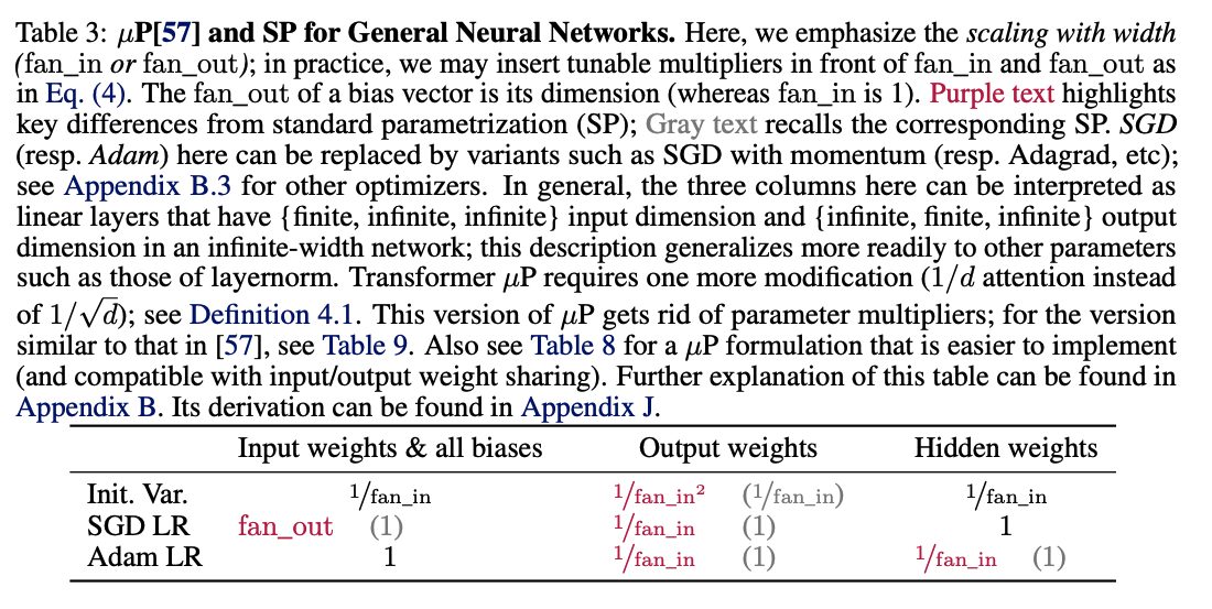
Comparing our results to Table 3 from tensor programs V (in which fan_in = n) looks like we derived the same results:
I want to thank Ilia Badanin and Eugene Golikov for helping me with this proof.